


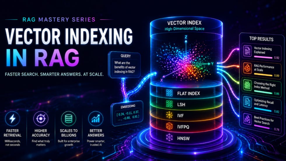
As Retrieval-Augmented Generation (RAG) systems grow from small prototypes into enterprise-scale platforms, one challenge quickly becomes impossible to ignore: retrieval performance. Storing millions of document chunks is easy. Finding the right ones in milliseconds is not. This is where vector indexing becomes a critical architectural decision. In this article, we explore the indexing techniques that power modern vector databases, compare their strengths and trade-offs, and examine why methods such as HNSW have become the default choice for production RAG systems. Whether you are building your first RAG solution or scaling to hundreds of millions of vectors, understanding vector indexing is essential to delivering fast, accurate, and cost-effective retrieval.
Why Indexing Matters
Indexing is how the embeddings inside a vector database are organized so that the retriever can find the most relevant items quickly and accurately. At small scale, the database can compare your query against every stored vector and still respond in milliseconds. At large scale, that brute force approach falls apart. A good index method makes retrieval fast without sacrificing too much accuracy. Notice the words fast and accurate. These two goals are in tension. Every index method is a different point on the tradeoff curve.
Traditional Databases Versus Vector Databases
In a traditional relational database, information is stored in rows with columns that provide metadata. Queries find exact matches or very similar matches by comparing values directly. The query for customer last name equals Smith is a deterministic lookup.
In a vector database, each document chunk is stored as an embedding that captures its meaning rather than its literal text. The query is also converted into an embedding, and the database returns the chunks whose embeddings are closest in meaning. This is semantic search. There is no exact match. There is only approximate nearness in a high dimensional space.
Because there is no exact match, the database needs a way to find the nearest neighbors without comparing the query against every vector in the store. That is what an index method provides.
Similarity Metrics, the Foundation
Before we discuss index methods, we need to be clear on how closeness is measured. Three metrics dominate the field.
1. Cosine Similarity
Measures the angle between two vectors and ignores their magnitude. Most common in RAG. Two pieces of text with similar meaning produce vectors that point in similar directions, regardless of length. This metric is robust against differences in text length, which is why it is the workhorse choice for most embedding models.
2. Dot Product
Combines direction and magnitude. Useful when the magnitude itself carries information, which is true for some embedding model families. Some models are trained specifically for dot product retrieval and produce embeddings normalized for this purpose.
3. Euclidean Distance
The straight line distance between two points in vector space. Geometrically intuitive but sensitive to magnitude. Used less often in modern RAG than cosine or dot product.
The choice of similarity metric should match the choice of embedding model. Check the model card. If the documentation says the embeddings are optimized for cosine similarity, use cosine similarity.
The Five Index Methods You Need to Know
1. Flat Index
How it works:the simplest approach. Each chunk is converted into an embedding and stored as is. On query, the query embedding is compared against every embedding in the database.
Strength:highest possible accuracy. Nothing is approximated. The nearest neighbors returned are guaranteed to be the true nearest neighbors.
Limitation:prohibitively slow at scale. Every query scans the entire dataset. Fine for thousands of vectors. Painful at millions. Unworkable at hundreds of millions.
When to use:early prototyping, small private knowledge bases, or evaluation pipelines where you want a ground truth baseline.
2. Locality Sensitive Hashing (LSH)
How it works:vectors are grouped into buckets using specialized hash functions designed to map similar items to the same bucket. On query, the query vector is hashed the same way to identify the most similar buckets, and only the vectors inside those buckets are searched.
Analogy:a library where books are categorized into broad sections, so you browse only the relevant section instead of the entire library.
Strength:fast bucket lookup. Lower memory footprint than graph based approaches.
Limitation:accuracy depends heavily on the quality of the hash functions. Poorly designed hashes lead to relevant items landing in unrelated buckets.
3. Inverted File Index (IVF)
How it works:groups vectors using clustering rather than hashing. The dataset is partitioned into dense groups based on resemblance, and a centroid is computed for each cluster. On query, the system identifies which clusters are closest to the query and searches only inside those.
Strength:much faster than Flat. Good for moderate scale knowledge bases.
Boundary problem:when a query lies near the boundary between several clusters, the system may need to search multiple clusters, which adds latency. Tuning the number of clusters and the number probed per query is a familiar IVF chore.
4.Inverted File Product Quantization (IVFPQ)
How it works:improves on IVF by further compressing the vectors. Each vector within a cluster is broken down into smaller sub vectors, and those sub vectors are encoded into compact bit representations through product quantization. Comparisons during retrieval are performed on these compact codes rather than full precision embeddings.
Strength:very memory efficient and dramatically faster comparisons. Crucial when you have to fit hundreds of millions of vectors on a constrained hardware budget.
Limitation:a small accuracy loss from quantization. Acceptable in most enterprise contexts but worth measuring.
5. Hierarchical Navigable Small Worlds (HNSW)
How it works:builds a graph with multiple layers. When a document is added, it begins at the top layer of the graph and is connected to its nearest neighbors in each layer it traverses. Each node is linked to its nearest neighbors, forming a multi layered structure. On query, search begins at the top layer, finds the nearest neighbor, and moves down through successive layers, narrowing the search at each step. At the bottom layer, the search returns the most similar vectors.
Strength:the most popular indexing method in production today because it is both fast and accurate. By moving from coarse to fine across layers, HNSW eliminates the vast majority of the dataset from consideration in a small number of steps.
Tradeoff:higher memory footprint than IVFPQ and tuning the graph parameters can be intricate. Most teams accept the memory cost in exchange for the latency and accuracy benefits.
Indexing Methods at a Glance
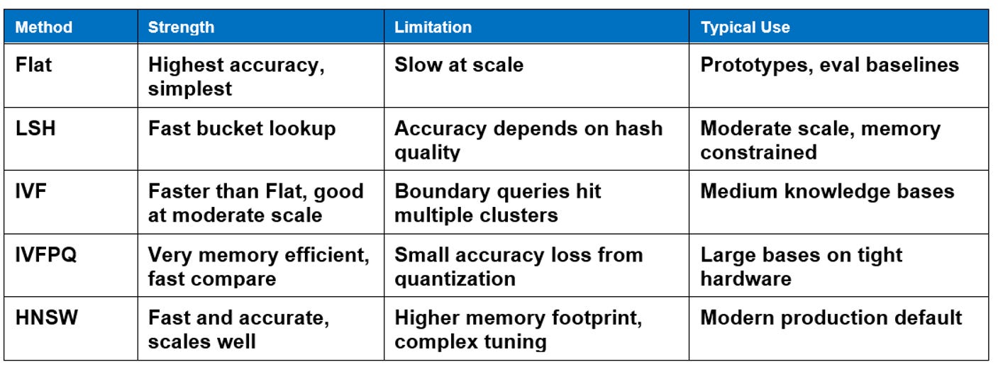
Indexing Methods at a Glance
Index choice is necessary but not sufficient. Several techniques layer on top to lift retrieval quality further.
1. Query Enrichment
Short or vague queries embed poorly. Prompt the user or the system to enrich the query with extra context before embedding. A two word question becomes a fuller paragraph that produces a much better query vector.
2. Hybrid Retrieval
Combine semantic vector search with traditional keyword search, often using BM25 for the keyword side. Vector search catches paraphrases and conceptual matches. Keyword search catches exact terms, proper nouns, and codes that embeddings sometimes blur. Hybrid retrieval is now the default in serious production stacks.
3. Reranking
After initial retrieval returns a candidate set, a smaller, more accurate model rescore the candidates and reorders them. Reranking consistently improves retrieval precision and is one of the highest leverage and lowest cost optimizations available.
4. Multi Scale Tree Graphs and Specialized Methods
For specialized use cases, hierarchical tree structures and other advanced graph methods can outperform HNSW on specific data shapes. Most teams should not start here. Start with HNSW and hybrid retrieval and earn the right to optimize further by measuring.
Mature Platforms You Will See in Vendor Conversations
ChromaDB,lightweight, developer friendly, popular for prototyping.
Pinecone,fully managed, strong on enterprise features such as access control and metadata filtering.
Weaviate,open source with hybrid search built in and a strong schema model.
Milvus and Zilliz,open source and managed flavors, used at large scale.
Qdrant,open source, Rust based, growing fast in production.
pgvector for Postgres, OpenSearch, Elasticsearch,vector capabilities increasingly built into the databases you already run, which simplifies operations.
Frameworks like LlamaIndex and LangChain sit above the database and abstract many of these choices.
A Sensible Default for 2026 Production
If you are starting a new RAG project today and you do not have a compelling reason to choose otherwise, the safe defaults are:
HNSW for the index.
Cosine similarity for the metric.
Hybrid retrieval with a sparse partner like BM25.
A cross encoder reranker between retrieval and generation.
Metadata filtering for governance and access control.
That configuration is enough to take most enterprise RAG projects from prototype to production. You can earn the right to optimize each piece by measuring.
Closing Thought
Indexing is one of those engineering choices that looks abstract until it bites you. The moment your knowledge base outgrows a single server and your latency budget tightens, the right index method is the difference between a system people use and a system people avoid.
In Part 6, we will turn to the hardest and most overlooked discipline in RAG: Evaluation. Without it, you cannot tell whether any of these choices are actually helping.

Explore more: Start Here · Topics · Archive · About